Example of usage of BioSSA & reconstruct functions
- “read.emb.data” reads 2d data from file and returns data frame
- “BioSSA” constructs a new BioSSA decomposition object from passed embryo object or formula
- First argument of “BioSSA” is formula evaluated with using data
- L is the window length
- step is the grid step of interpolation
- xlim and ylim are cutoff bounds by AP and DV axes
- xperc and yperc denotes the size (width and height) of presented embryo part in percent
xlim <- c(22, 88)
ylim <- c(32, 68)
L <- c(15, 15)
file <- system.file("extdata/data", "ab16.txt", package = "BioSSA")
df <- read.emb.data(file)
bss <- BioSSA(cad ~ AP + DV, data = df,
L = L,
step = 0.5,
xlim = xlim, ylim = ylim)
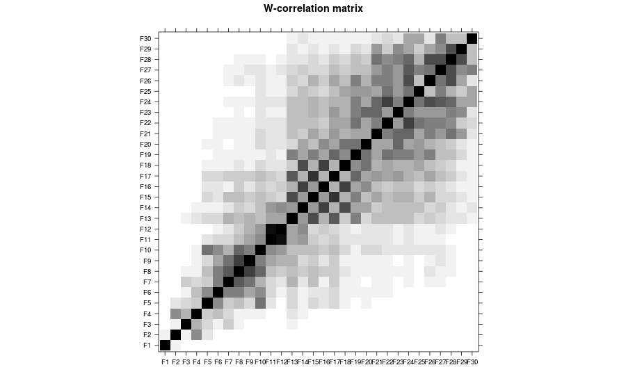
# w-correlations for identification
plot(plot(bss, type = "ssa-wcor", groups = 1:30))
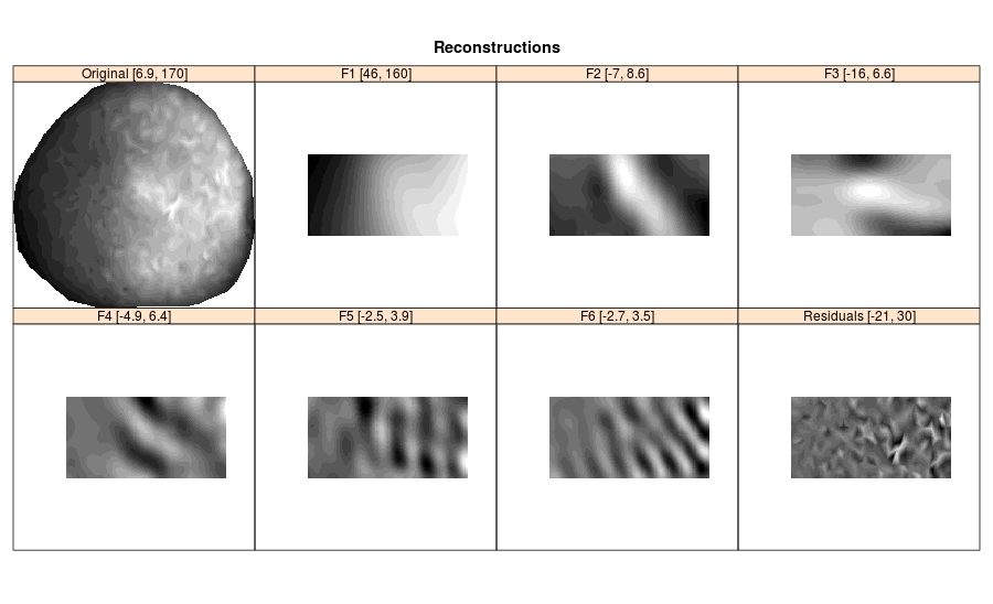
# Reconstruction of elementary components
rec.elem <- reconstruct(bss, groups = 1:6)
plot(plot(rec.elem))Produced output
Checking of decomposition quality
bad <- 1
good <- 3
wave <- 3
atx <- 50
aty <- 50
tolx <- 5
toly <- 5
ylim1 <- c(-10, 10)
ylim2 <- c(-1, 1)
ylim3 <- c(-0.2, 0.2)
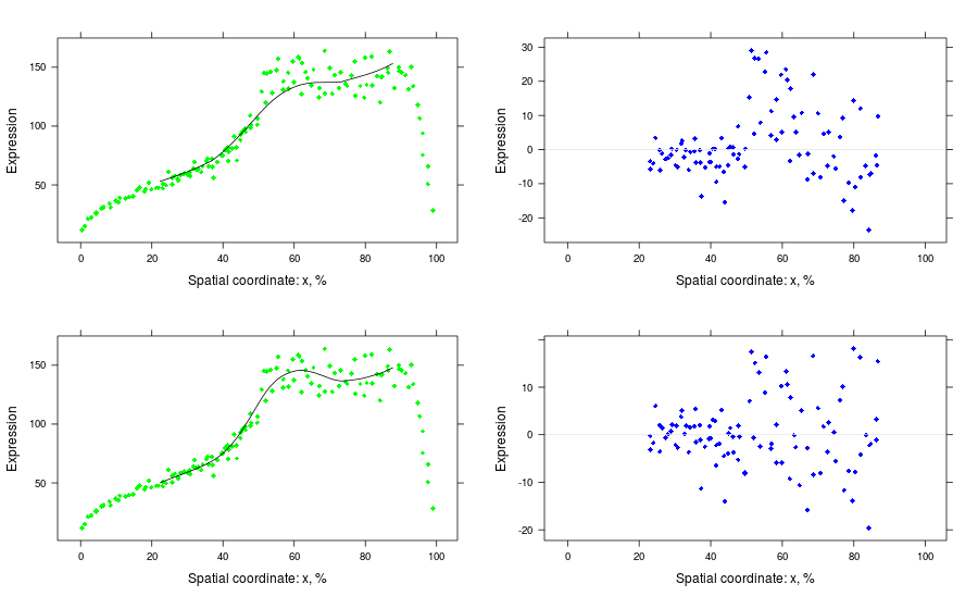
# Sections for testing the reconstruction quality
rec <- reconstruct(bss, groups = list(good = 1:good, bad = 1:bad))
p.ny <- plot(attr(rec, "series"), type = "nuclei-section", at = aty, coord = "y", tol = toly)
p.fy1 <- plot(rec$bad, type = "field-section", at = aty, coord = "y")
p.fy2 <- plot(rec$good, type = "field-section", at = aty, coord = "y")
p.nx <- plot(attr(rec, "series"), type = "nuclei-section", at = atx, coord = "x", tol = tolx)
p.fx1 <- plot(rec$bad, type = "field-section", at = atx, coord = "x")
p.fx2 <- plot(rec$good, type = "field-section", at = atx, coord = "x")
# y-sections, bad and good
pls <- list()
pls[[1]] <- p.ny + p.fy1
pls[[2]] <- plot(residuals(bss, 1:bad), type = "nuclei-section",
at = aty, coord = "y", tol = toly,
ref = TRUE, col = "blue")
pls[[3]] <- p.ny + p.fy2
pls[[4]] <- plot(residuals(bss, 1:good), type = "nuclei-section",
at = aty, coord = "y", tol = toly,
ref = TRUE, col = "blue")
print(pls[[1]], split = c(1, 1, 2, 2), more = TRUE)
print(pls[[2]], split = c(2, 1, 2, 2), more = TRUE)
print(pls[[3]], split = c(1, 2, 2, 2), more = TRUE)
print(pls[[4]], split = c(2, 2, 2, 2))
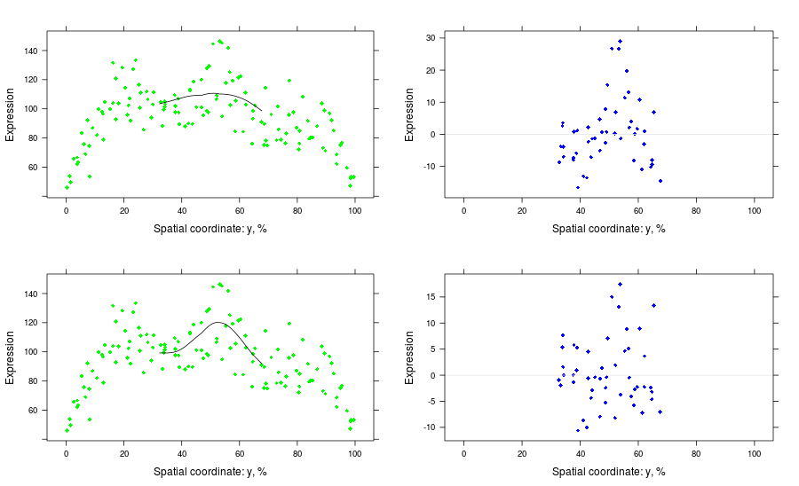
# x-sections, bad and good
pls <- list()
pls[[1]] <- p.nx + p.fx1
pls[[2]] <- plot(residuals(bss, 1:bad), type = "nuclei-section",
at = atx, coord = "x", tol = tolx,
ref = TRUE, col = "blue")
pls[[3]] <- p.nx + p.fx2
pls[[4]] <- plot(residuals(bss, 1:good), type = "nuclei-section",
at = atx, coord = "x", tol = tolx,
ref = TRUE, col = "blue")
print(pls[[1]], split = c(1, 1, 2, 2), more = TRUE)
print(pls[[2]], split = c(2, 1, 2, 2), more = TRUE)
print(pls[[3]], split = c(1, 2, 2, 2), more = TRUE)
print(pls[[4]], split = c(2, 2, 2, 2))
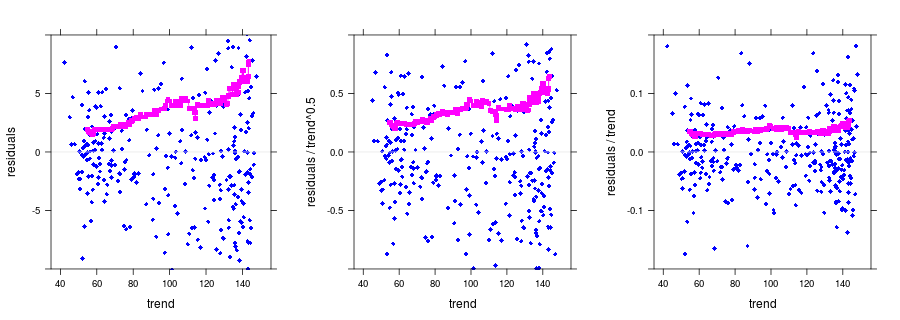
#dependence of noise on trend
nm.add <- noise.model(bss, groups = 1:good, model = "additive")
nm.pois <- noise.model(bss, groups = 1:good, model = "pois")
nm.mult <- noise.model(bss, groups = 1:good, model = "mult")
p1 <- plot(nm.add, ylim = ylim1, print.alpha = FALSE)
p2 <- plot(nm.pois, ylim = ylim2, print.alpha = FALSE)
p3 <- plot(nm.mult, ylim = ylim3, print.alpha = FALSE)
print(p1, split = c(1, 1, 3, 1), more = TRUE);
print(p2, split = c(2, 1, 3, 1), more = TRUE);
print(p3, split = c(3, 1, 3, 1));Produced output