Example of BioSSA application

Decomposition of cylindrical data

Let us consider data for expression of gene activity measured on the embryo of the drosophila (fruit fly). The form of the embryo is similar to ellipsoid and therefore the cylindrical projection is adequate for a middle part of the embryo. The technique of SSA analysis of such kind of 2D data by planar non-shaped 2D-SSA was developed in Golyandina et al (2012) and Holloway et al (2011). After projection, the initial data given on 3D embryo surfaces are represented in the form \((x_i, y_i, f_i)\) where \((x_i, y_i)\) are coordinates of nuclei centers in the cylindric projection transformed to a planar rectangle, \(f_i\) are the expression values. The aim of the analysis is to decompose data into a sum of pattern and noise and then measure the signal/noise ratio. Data are cropped and then are interpolated to a regular grid; therefore, we obtain a digital image, which can be processed by 2D-SSA. Values of smoothed expression are interpolated backward onto nuclei centers.

Here we demonstrate that the developed circular version of 2D-SSA can perform smoothing without artificial transformation of a cylinder to the rectangle. Thus the result of processing does not depend on the technique of this transformation and has no extra edge effects. We consider the cylindrical topology.

Data were downloaded from the BDTNP archive, the file “v5_s11643-28no06-04.pca”.

Data on the surface of embryo are given in 3D coordinates, therefore we calculated cylindric coordinates by finding the principal axis of the data. The interpolation is performed with the step 0.5% and the middle part from 20 to 80% of the embryo lengths were processed.

The result of decomposition (the factor vectors from the \(12\) leading eigentriples) is depicted in the figure below.

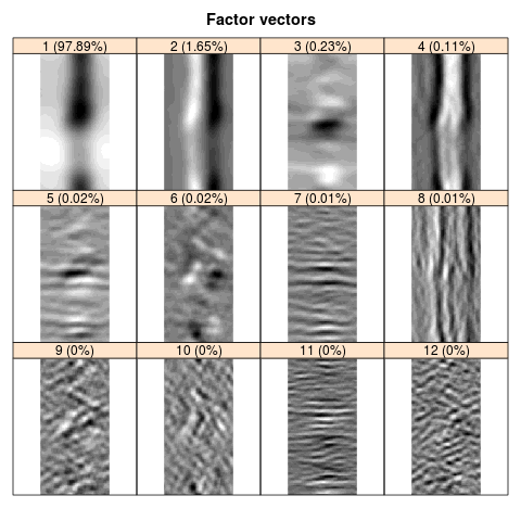
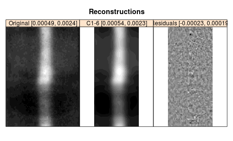
The components 1-6 grouped together provide an adequate smoothing; the residual oscillates around zero. Note that the bottom and top edges are coincide, that is, there is no edge effect.

Construction of noise model

In this section we consider the problem of construction of the noise model, see Noise Model for a theory and Noise estimation example for a code. We again investigate data for expression of gene activity measured on the embryo of the drosophila (fruit fly) but the data are 2D.

Logic of the investigation is as follows:

1. To start with, we choose parameters for SSA based on the 2D-SSA theory and sizes of the embryo.
2. Then we check that the result of reconstruction is adequate by means of 1D profiles.
3. Then the multiplicity parameter \(\alpha\) is estimated and the conclusion based on its value is performed: 0 corresponds to the additive model of noise, 0.5 reflects a Poissonian nature of the noise and 1 corresponds to the multiplicative model.

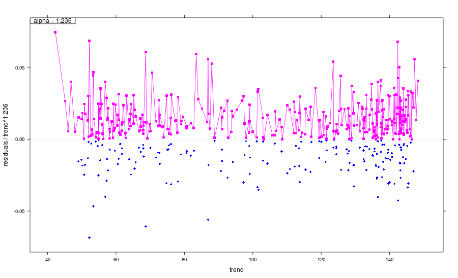
The following example produces the estimate \(\alpha = 1.236\), which shows that the model is rather multiplicative:

Noise model:
  Multiplicity: 1.236 
  sigma: 0.009559 
  Noise sd: 0.0207